The last time we analyzed a system dynamics model, it was easy with just 1 stock, 2 flows, and 2 variables. The relationships between variables were very straightforward and simple. This time, we take another 1-stock system, but we try to go and model tinier details in an attempt to make the model as close to reality as possible. Note that we can only aim to create a model which reflects reality perfectly; however, any model, at best, is an approximation of real-world phenomena, however accurate enough to be used for producing meaningful results.

As an example problem, let’s try and model a bank account. Here, we consider the bank account to be the stock, which maintains a record of the amount of funds available in the account - or in layman’s terms, the bank balance. Take a look at the model below; we will then dissect it piece by piece, analyze the important traits and perform some simulations.

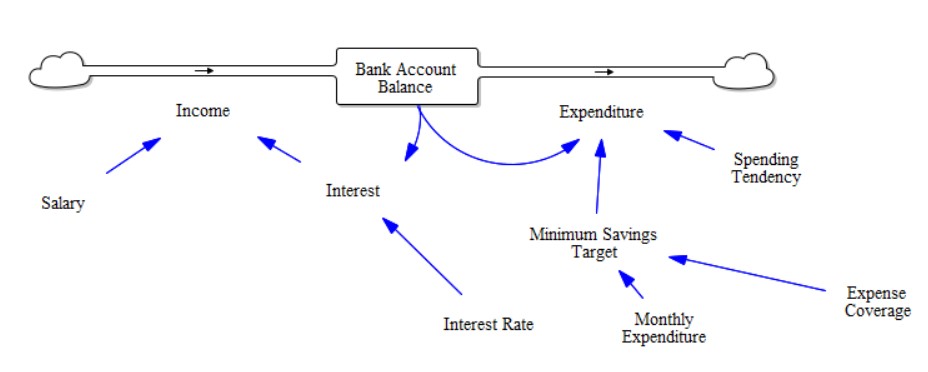
Before going on to simulations, let’s take a detailed look at the model components.

Model Description

Sr. No	Component Name	Short Name	Component Type	Units	Expression	Initial Value	Explanation
1	Bank Account Balance	BAB	Stock	$	\(\int(Income - Expenditure)\)	100	Records the available account balance
2	Expenditure	EXP	Flow	$/month	IF THEN ELSE ((BAB-MINSAVTGT)>0, (BAB-MINSAVTGT)XSPENTEND + MONEXP, MONEXP	NA	records monthly expenditure
3	Expense Coverage	EXPCOV	Variable	month	12	NA	Duration for which the current balance should suffice wrt to basic monthly expenditure
4	Income	INC	Flow	$/month	SAL + INT		Records monthly income from all sources
5	Interest	INT	Variable	$/month	\(\frac{BAB \times INTRT}{100}\)		Registers principal interest gained from bank for savings
6	Interest Rate	INTRT	Variable	1/month	0.33		Rate of interest the bank offers for savings account
7	Minimum Savings Target	MINSAVTGT	Variable	$	EXPCOV*MONEXP		Minimum amount of bank balance to cover basic monthly expenditure for EXPCOV amount of duration
8	Monthly Expenditure	MONEXP	Variable	$	20		Registers monthly expenditure
9	Salary	SAL	Variable	$/month	50		Registers amount of salary earned per month
10	Spending Tendency	SPENTEND	Variable	Dimensionless	0.15		Records the spending tendency of the account owner - the higher the value, the higher the user’s spending - this acts as a multiplier and hence is dimensionless

Although we could make a simple model based on income and expenditure where the flows are independent of the stock, we add an additional complexity to take the model closer to reality. So in our model, the inflows and outflows both are dependent on the stock levels. If you think about it, then it makes sense, isn’t it? Everyone only spends as much as they can earn back - if someone earns more, they can afford to spend more. Also, everyone (okay, every rational human being lol) maintains a target of savings to fend for basic needs like housing, clothing, food, medical emergencies, et al., for some duration of time - in case any untoward event happens, like if they lose their job, or their employer closes down.

Observe the figure carefully. The total amount of interest earned on the savings depends on the ‘Rate of Interest’ and the bank balance. This leads to a reinforcing feedback loop, provided the interest rate is kept constant, interest getting deposited back to the balance creates more interest, which in turn increases the balance, giving rise to an exponential growth tendency. On the other hand, the expenditure loop is a balancing loop, i.e., the higher the difference between bank balance and minimum savings target, the higher expenditure is - which in turn causes a reduction in the bank balance, which in turn causes a reduction in expenditure in the next iteration. So this acts as a balancing loop - though here, it doesn’t directly depend on the bank balance but on various other factors as well.

What did we miss?

Here, it should be stated that the model is not perfect – it doesn’t accurately match reality. In reality, the interest rate offered by the bank depends on the financial performance of the bank and other market conditions. In the real world, the salary doesn’t remain constant, but people get annual increments; hence their salary keeps increasing. So, in a level up from this model, we can consider salary as another stock. We haven’t considered inflation at all, which has a prominent influence on expenditure. With increasing inflation, the monthly expenditure will increase, which we haven’t accounted for in the model. Again the spending tendency, which is assumed to remain constant, can increase based on financial security. The higher the financial savings one has - the higher the tendency that person will have to spend the excess income after they have left some aside for the essential expenditure - which we haven’t accounted for in our model. Hence you should never forget that any model is but an approximation of real-world phenomena, and the results it produces shouldn’t be used blindly to make forecasts and predictions. They should be used as a guidebook - but independent thought should be put in before using the results.

Model Simulation

Here is how the bank balance stock and the income and expenditure flows behave with time.

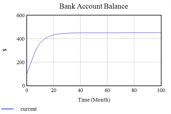
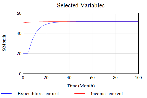
If you observe the trends, the bank balance increases and then stabilizes at a certain level. Similarly, the income and expenditure flow too stabilize at a particular level - equal to each other. Because they are stabilizing at the same level - the magnitude of inflow and outflow is equal, and the system is in a dynamic equilibrium. If you have studied linear control theory, then you will know that this response is very similar to the first-order system. When the output is affected by the input to the first order.

Now, here are some tasks for you to try out. Vary the parameters from the model: try setting the spending tendency to zero, or you can set the interest rate at a higher value and then check how the system behaves.

Don’t over-rely!

Now, in the case of simple systems, we can use common logic and overall system sense to qualitatively predict results based on the model. So you don’t always need to simulate the model.

1. Say the spending tendency is now set to zero. What is likely to happen? So since the spending tendency is set to zero, the expenditure will always be zero. So there, the bank balance stock will always keep increasing and won’t stabilize at any value.
2. If you increase the interest rate, then the overall general system behavior is similar. However, the bank account balance now stabilizes at a higher value.
3. Now, assume the monthly expenditure increases - what will happen? First of all, how will you model this change? Will you change the variable expression, or would you introduce a new stock for the monthly expenditure? How will the stock change - can you use inflation data to somehow realistically predict the increase the expenditure? Think about it and try it out on your own.

Here’s a result of the bank balance stock and income expenditure flows when the interest rate was 4pcpa and 8pcpa, respectively.

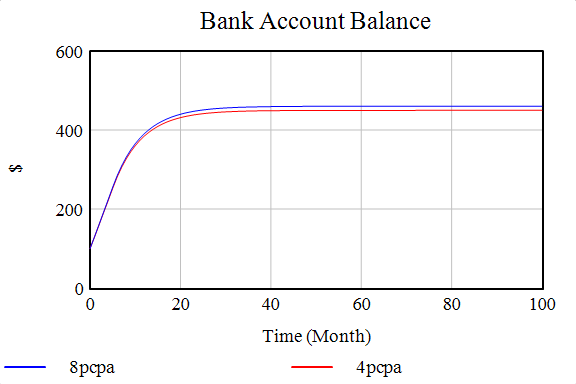
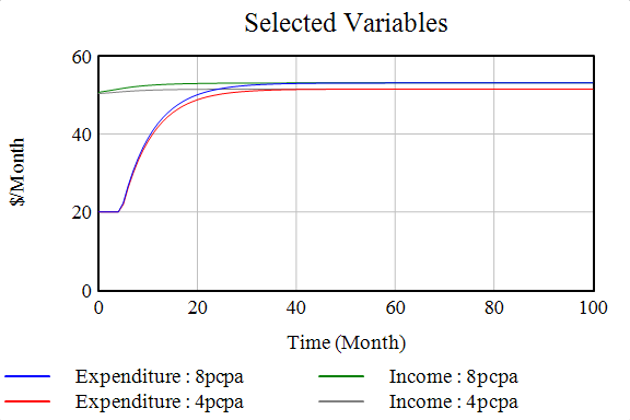
If you observe neatly, the bank balance in the case of an 8pcpa interest rate is higher than the 4pcpa case. In the expenditure case, you can see a constant graph in the initial months; you might wonder why - its because in the expression of expenditure, we had put in the condition that if the bank balance is less than the monthly savings target, then there will be no excess expenditure - leisure spending, but in any case, the essential monthly expenditure for housing, food, clothing - the bare necessities has to be done. Hence the plateau corresponds to the bare minimum expenditure, and in that duration, the bank balance is less than the monthly savings target. “So here we captured the reality that the expenditure can never be zero.” In the income and expenditure cases too, the settle at a higher value when the interest rate increases.

That’s it for this time, lads! Next time, we will look at more involved systems and real-world case studies! Till then, Saayonaara!

• Home Page
• « Previous Article (Causal Loop Diagram)